Complete Risk and Portfolio Theory in Math, Excel, Python — Magic Behind 329% Profit or 1000% Sharpe Ratio

16 min readNov 4, 2020

Summary and Results:

In 1 to 2 year short term, it is possible to find -30% negatively correlated Nasdaq stocks and achieve 1000% Sharpe ratio. But some correlations are spurious and need to be further vetted. As look back increases to before 2008, minimum correlation and Sharpe ratio decreased to 0.03 and 0.18 respectively. Considering multi-way correlation is also interesting and will be included in the future studies.
Enabling short sell of stocks pushes the efficient frontier up about 20% with the same risk; trading in risk-free-rate margin pushes the efficient frontier up by about 3% with the same risk.
Doing the same analysis for world’s 8 biggest equity indexes GSPTSE, FCHI, GDAXI, N225, FTSE, GSPC, AORD, HSI reveal that we should only invest in Hong Kong and UK post COVID if believing we are affected equally by the past events, also trusting Markowitz’s portfolio theory.
Clarify the concepts on the Capital Allocation Line where I think the textbooks failed to convey.
Send me private message to request for full version of the code or excel, as I was having some difficulty uploading them.
In the conclusion section, I demonstrated how to achieve 329% annual profit with the techniques covered in this educational and research oriented article. And the catch of all the things.

Introduction:

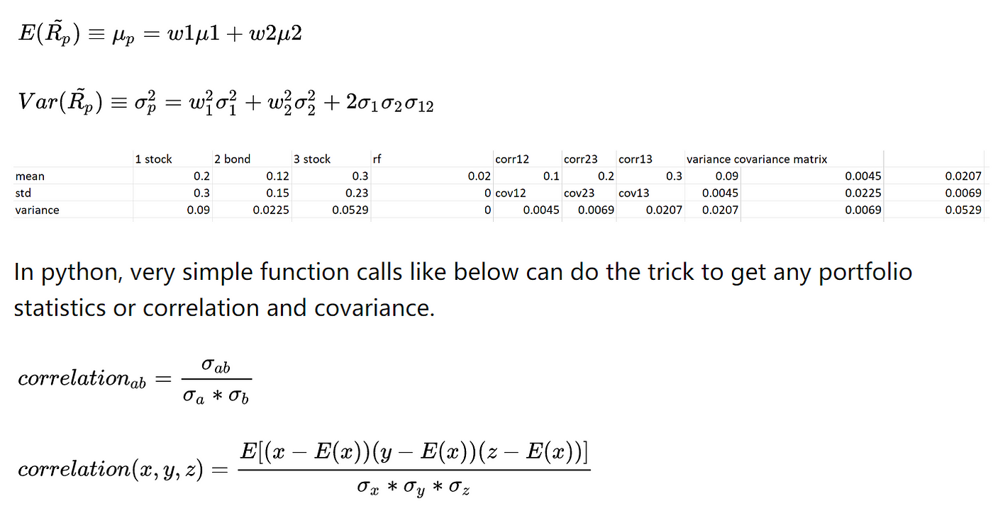
Under the mean-variance framework, the goal is to minimize the portfolio variance or volatility as much as possible. As the best economic decisions occur in margin, then portfolio is not optimal if one sub-asset can achieve more return than the other with marginal increase of portfolio risk (or volatility). This is called the Markowitz portfolio efficient frontier. The key here is the covariance; however, total diversification can only be as good as the market index. In order to conduct the analysis accurately, I first assume each stock’s return has normal distribution. Therefore, collectively we have multivariate normal distribution. The optimization problem only comes in when we want to minimize the variance or maximize the Sharpe ratio with certain constraints like portfolio weights or fixed expected returns.

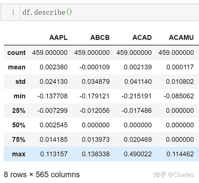
Step1: Determine the scope of securities in the portfolio to invest and calculation the basic statistics

I used all Nasdaq stocks from 2007 to 2020 as my base. See the Python code and comments near the end of this post for the details of my data, how I washed it, and what are the filters.

We could use that to vet our strategy beforehand.

df.describe()
df.corr().unstack().sort_values(kind='quicksort').drop_duplicates()
df.cov()

For example, I had generated below results for different periods. It is surely interesting to think about if you have in mind that lack of correlation does not imply independence, and the spurious correlation.

ACAD  SPNS    0.032700 <- least correlation between 2007 to 2020

Green is positively correlated with SPY, red is negatively correlated with SPY for each asset.

LRCX  AMAT    0.800469 <- strongest correlation between 2007 to 2020

CTXS  JBLU    -0.052000 <- least correlation between 2019 to 2020

AMAT  LRCX    0.923048 <- strongest correlation between 2019 to 2020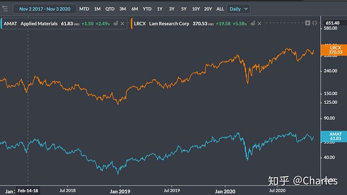

We can see the beta risk with SPY is not avoidable.

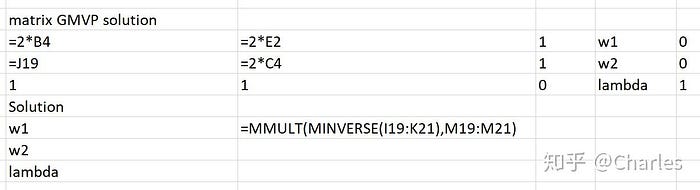
Step2: Minimizing the Lagrangian

Therefore, it is called an augmented matrix which should always have positive definite when we combine the partial derivatives of variance with respect to weights, with the 1’s and 0’s. The 2’s are resulted from taking the partial derivatives of sigma squared. 0 is given to the lagrangian multiplier.

Above list of linear equation is exactly the same as below matrix equation, which we can solve it with the inverse of augmented matrix.

After that, plugging the weights to expectation and variance will give the single global minimum variance portfolio point.

In python, ‘np.dot’ assembles ‘mmult’ function in excel. w’Σw is the function we want to minimize.

np.sqrt(np.dot(weights.T, np.dot(df_invest.cov(), weights)))

Then I used the scipy to do the optimization.

optimal_variance=optimize.minimize(minimize_volatility,initializer,method='SLSQP',bounds=bounds,constraints=constraints)

With the following parameters to do our 2D search.

# Initialize optimization parameters
constraints = ({'type' : 'eq', 'fun': lambda x: np.sum(x) -1}) # sum of weight is 1
# portfolio short-sell ss configuration
bounds = tuple((-1,1) for x in weights) # weights as defined earlier was already set for each asset column
# start from equally weighted for 2D optimization, risk and return
initializer = len(df_invest.columns) * [1/len(df_invest.columns)] # constant times an array

Same idea can be used for the maximum Sharpe ratio portfolio., which means the highest reward to any marginal change of variability. It may not have minimal risk; however, it is the most efficient and cost-effective with our past residual alpha’s.

Step3: Construct the efficient frontier

For two risky assets, due to fixed covariance measure, all the portfolio weight combinations lie on the efficient frontier, assuming we invest all the money given. However things get tricky when we have multiple risky assets and an entire variance-covariance matrix to calculate the investment opportunity set. Therefore, we need to add a second lagrangian multiplier for a set of fixed expected return starting after the global minimum variance point, and find the least variance point for them. Connecting all the min variance portfolios will give us efficient frontier.

It looks like this in excel:

And more or less the same idea in python for using linearly spaced returns and calculate each minimum variance portfolio in a ‘for’ loop. One thing to note is that if each optimization takes 10–20 minutes, finding the minimum variance efficient frontier can take hours. However, this is still very fast to compute huge matrices compare to old unprivileged times.

target_returns = np.linspace(port_returns.min(),port_returns.max(),1)# Initialize optimization parameters
minimal_volatilities = []for target_return in target_returns:
    # for graphing the frontier, this time we added 1 more constraint besides sum weight=1, which is the expected return formula
    constraints = ({'type':'eq','fun': lambda x: portfolio_stats(x)['return']-target_return},{'type':'eq','fun': lambda x: np.sum(x)-1})
    optimal = optimize.minimize(minimize_volatility,initializer,method='SLSQP',bounds=bounds,constraints=constraints)
    minimal_volatilities.append(optimal['fun']) # this give the x axis
    
minimal_volatilities = np.array(minimal_volatilities

Eventually, it can be proved that all the outcome of weights should be linear dependent.

Step4: Tangent portfolio and capital allocation line

We can consider tangent portfolio as a risky portfolio consisting whichever number of risky asset plus another portfolio of pure risk-free instruments.

Margin Purchase and Short Selling

This is the graph representing the combination of a risky portfolio and a riskless portfolio gotten from above excel formulas.

Each security can weigh from 0 to 1.

Each security can weigh from -1 to 1.

The Utility Function

In the utility function under prospect theory, x axis is the change of wealth and y axis is the utility, which can also be thought as investor’s achieving goal.

Following graph represents the Jensen inequity.

Since portfolio expectation and variance are formulae of weight in risky and riskless assets. Given the utility function, I can optimize y (weight in risk-free portfolio in screenshot) to maximize my utility.

Python code

%%time
import yfinance as yf
import os
import sys
print(os.getcwd())
#print(sys.path)
print(os.__file__)
%matplotlib inline
%config InlineBackend.figure_format = 'retina' 
import matplotlib
import matplotlib.pyplot as plt
import io, base64, os, json, re
import pandas as pd
import numpy as np
import datetime as dt
import seaborn as sns
import scipy.optimize as optimize
pd.set_option('display.max_rows', 500)
from pandas_datareader import data as pdr
from pandas.plotting import scatter_matrix
from scipy.stats import variation, norm
import time
import scipy.interpolate as sci

This is how I got all the Nasdaq stock tickers to the “companylist.csv” from Nasdaq api.

# # download tickers from weblink
# %%time# import pandas as pd
# import requests
# import io# url = 'https://old.nasdaq.com/screening/companies-by-name.aspx?letter=0&exchange=nasdaq&render=download'
# r = requests.post(url)
# if r.ok:
#     data = r.content.decode('utf8')
#     df = pd.read_csv(io.StringIO(data))
# df.head()

I only picked stocks in the billions market cap range, filtered all the ‘NA’, and only those have at least a year of historical data. It turned out that I filtered from 3849 to 644 names, which is plenty for the analytics.

%%time
tickers_df = pd.read_csv('companylist.csv')
print(len(tickers_df))
tickers_df = tickers_df.loc[tickers_df['MarketCap'].str.contains(r'B',na=True)]
print(len(tickers_df))
tickers_df = tickers_df.dropna(subset=['Sector','industry','LastSale','IPOyear'],axis=0,how='any')
print(len(tickers_df))
tickers_df = tickers_df.loc[tickers_df['IPOyear']<2020]
print(len(tickers_df))
tickers_df

Next is to download the historical data from yahoo, clean the data, get the log returns. You could also use simple returns, depending on your understanding of whether things are generally growing exponentially or not. Here I picked my data from 2019–01–01 to 2020–10–25 for historical beta look back. I agree this could be more rigorous; however, it is subjected to mroe complex time series analysis in the future. Note all the current portfolio construction theories or regression models do not predict alpha! Beta is predictable if you assume historical events have equally weighted influence on future events.

%%time
# get tickers from csvtickers_list = tickers_df.iloc[:,0].tolist()
tickers_str = " ".join(tickers_list)
tickers_str%%timeyf.pdr_override() 
# download dataframe
data = pdr.get_data_yahoo(tickers_str, start="2019-01-01", end="2020-10-25")["Adj Close"] # history lookback configuration# same data if rerun
data_save = data
data%%time
# clean data
data = data.dropna(axis=1,how='all')
data = data.fillna(method='ffill')
data = data.fillna(method='bfill')
data%%time
# change price to log returndf = pd.DataFrame() 
for i in data:
    if i not in df:#so rerunning the cell will not double add
    # Calculates the difference of a Dataframe element compared with another element in the Dataframe (default is element in previous row).
        df[i] = np.log(data[i]).diff() 
df = df[1:]
df# # if want to graph
# scatter_matrix(df,figsize=(10,10),alpha=0.5)
# sns.heatmap(df.corr(), annot=True, fmt='.1g',cmap=plt.cm.Blues) 
# plt.show()

Then we try to find series of correlation between two elements.

%%time
# print(df.corr().idxmin(axis=0))
df.corr().unstack().sort_values(kind='quicksort').drop_duplicates()

Wall time: 380 ms
NFINU  LOACU   -0.394853
CFFAU  MCRB    -0.292155
WDFC   KBLMU   -0.290402
BNTX   PENN    -0.281356
GMHIU  SRACU   -0.274526
                  ...   
COLB   HOMB     0.882085
IBTX   TCBI     0.887901
FIBK   SFBS     0.891678
AMAT   LRCX     0.923048
AAPL   AAPL     1.000000
Length: 159331, dtype: float64

Here is our sample data statistics. Note the mean is the alpha here.

%%time
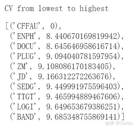
# find coefficient of  variation for dispersion of the distribution in relation to the mean
# lower CV should be better than higher cv in generalstd_dict={}
for i in df.columns:
    std_dict[i]=np.std(df[i])mean_dict={}
for i in df.columns:
    mean_dict[i]=np.mean(df[i])cv_dict={}
for i in df.columns:
    cv_dict[i]=std_dict[i]/abs(mean_dict[i]) if abs(mean_dict[i]) != 0 else 0
    
display(sorted(std_dict.items(),key=lambda x: x[1],reverse=True)[:5])
display(sorted(mean_dict.items(),key=lambda x: x[1],reverse=True)[:5])
display(sorted(cv_dict.items(),key=lambda x: x[1],reverse=True)[:5])

Now it is time to construct our own portfolio. We define the investment amount, confidence interval for VAR calculation, and for example below code extract assumes we only use the top 5 stocks alphabetically.

%%timeinvestment = 10000 # 10k usd
confidence = 0.05 # The interval has an associated confidence level that the true parameter is in the proposed range.
################################# investing portfolio configuration
#df_invest = df.iloc[:,0:10] # choose how many stocks in our investing portfolio
df_invest = df.iloc[:,0:5] 
###################################
weights = np.array(len(df_invest.columns) * [1/len(df_invest.columns)])
print(weights)
display(df_invest.cov())
print(len(np.mean(df_invest)))
print(len(weights))
portfolio_mean_pct_return = np.mean(df_invest).dot(weights) #this means sum product of 2 arrays not matrix dot multiplier
print('mu is '+str(portfolio_mean_pct_return))
portfolio_std_pct_return = np.sqrt(weights.T.dot(df_invest.cov()).dot(weights )) #w'.SIGMA.w
print('sigma is '+str(portfolio_std_pct_return))

And this is our covariance matrix:

Followed by VAR (value at risk) calculation:

So it becomes:

Absolute VaR = investment * [(z number under normal given confidence interval) * standard deviation of portfolio + expected return of portfolio]

Relative VaR = investment * [(z number under normal given confidence interval) * standard deviation of portfolio]

Absolute VaR is the total possible loss, and relative VaR is assuming we can get expected return. Therefore, relative VaR has a less negative number. If we need to scale with time, we need to multiply by the square root of time t. As volatility is the square root of variance only which is additive with respect to time. The concept is not the same as V(t*x)=t*V(x) in time series, where x is a function of t.

%%time
var_z = norm.ppf(confidence, 0, 1)
# ppf is the cdf or area under pdfnum_days = int(5)
for x in range(1,num_days+1):
# aV[x] = V[sqrt(a)*x]
# this is saying we are 95% confident that our portfolio of 10k USD will not lose more than the amount over next few days
    abs_var = np.round(investment*(var_z*portfolio_std_pct_return+portfolio_mean_pct_return)*np.sqrt(x),0) 
    relative_var = np.round(investment*(var_z*portfolio_std_pct_return)*np.sqrt(x),0)
    print(str(x)+' day absolute VaR @ 95% confidence: '+str(abs_var))
    print(str(x)+' day relative VaR @ 95% confidence: '+str(relative_var))

Then, we prepare for portfolio construction, simulation, and optimization.

%%time
#portfolio construction, simulation, and optimization
# this cell is for experimenting
'''
inear map [0,1] to [-1,1] to cope for short selling negative dirichlet distribution weights
I found a good way to do the transformation for dimension higher than 3 and posted on stackexchange
https://stackoverflow.com/questions/63910689/transformed-dirichlet-array-with-range-1-1-in-numpy/64656760#64656760
'''
weights = np.random.dirichlet(alpha=np.ones(len(df_invest.columns)), size=1) # generates a random array of weights for each asset that sum to 1 and assume all money will be deploye
weights = 1/(len(df_invest.columns)/3)-2*weights
print(weights,np.sum(weights))
weights = weights[0]
exp_port_return = np.sum(df_invest.mean()*weights) 
print('portfolio expected return in the period defined by me '+str(exp_port_return))port_var = np.dot(weights.T, np.dot(df_invest.cov(), weights))
port_vol = np.sqrt(port_var)
print('portfolio variance '+str(port_var))
print('portfolio risk or volatility '+str(port_vol))

Above is the bread and butter for our calculation assuming random weights. If considering short selling weights, we also need to linearly map the dirichlet distribution from [0,1] to [-1,1]. I use trial and error to find y=1/(dimension/3)-2*x transformation worked without needing to know the theory behind.

Transformed Dirichlet array with range [-1,1] in numpystackoverflow.com

%%time
def portfolio_simulation(assets, iterations): 
    start = time.time() 
    num_assets = len(assets) 
    port_returns = [] 
    port_vols = []
    for i in range (iterations):
        # linear map [0,1] to [-1,1] to cope for short selling negative dirichlet distribution weights
        weights =  1/(len(df_invest.columns)/3)-2*np.random.dirichlet(alpha=np.ones(num_assets),size=1)
        weights = weights[0]
        #print(weights) # this would print all iterations of weights
        # if sample days are too few, mean will be close to zero or less than zero. so frontier will have upper half missing
        port_returns.append(np.sum(df_invest.mean()*weights)) #same as using .dot() for sum product
        port_vols.append(np.sqrt(np.dot(weights.T, np.dot(df_invest.cov(), weights)))) #.dot() means matrix multiplication or sum product
    # Convert lists to arrays
    port_returns = np.array(port_returns) 
    port_vols = np.array(port_vols)
    # Plot the distribution of portfolio returns and volatilities
    plt.figure(figsize = (18,10))
    plt.scatter(port_vols,port_returns,c=(port_returns/port_vols),marker= 'o')
    plt.xlabel('Portfolio Volatility')
    plt.ylabel('Portfolio Return')
    plt.colorbar(label = 'Sharpe ratio (not adjusted for short rate)')
    print('Elapsed Time: %.2f seconds' % (time.time() - start))
    return port_returns, port_volsport_returns, port_vols = portfolio_simulation(df_invest.columns, 10000)Transformed Dirichlet array with range [-1,1] in numpy%%time
def portfolio_simulation(assets, iterations): 
    start = time.time() 
    num_assets = len(assets) 
    port_returns = [] 
    port_vols = []
    for i in range (iterations):
        # linear map [0,1] to [-1,1] to cope for short selling negative dirichlet distribution weights
        weights =  1/(len(df_invest.columns)/3)-2*np.random.dirichlet(alpha=np.ones(num_assets),size=1)
        weights = weights[0]
        #print(weights) # this would print all iterations of weights
        # if sample days are too few, mean will be close to zero or less than zero. so frontier will have upper half missing
        port_returns.append(np.sum(df_invest.mean()*weights)) #same as using .dot() for sum product
        port_vols.append(np.sqrt(np.dot(weights.T, np.dot(df_invest.cov(), weights)))) #.dot() means matrix multiplication or sum product
    # Convert lists to arrays
    port_returns = np.array(port_returns) 
    port_vols = np.array(port_vols)
    # Plot the distribution of portfolio returns and volatilities
    plt.figure(figsize = (18,10))
    plt.scatter(port_vols,port_returns,c=(port_returns/port_vols),marker= 'o')
    plt.xlabel('Portfolio Volatility')
    plt.ylabel('Portfolio Return')
    plt.colorbar(label = 'Sharpe ratio (not adjusted for short rate)')
    print('Elapsed Time: %.2f seconds' % (time.time() - start))
    return port_returns, port_volsport_returns, port_vols = portfolio_simulation(df_invest.columns, 10000)

We apply the bread and butter in the multiple iteration simulation to get the scatters of our possible portfolio weights.

%%time
def portfolio_stats(weights):
    # Convert to array in case list was passed instead.
    weights = np.array(weights)
    port_return = np.sum(df_invest.mean() * weights)
    port_vol = np.sqrt(np.dot(weights.T, np.dot(df_invest.cov(), weights))) 
    sharpe = (port_return-0)/port_vol # assume risk free rate is 0
    return {'return':port_return,'volatility':port_vol,'sharpe':sharpe}# this is when slope of the efficent frontier is highest
def minimize_sharpe(weights): #minimize negative sharpe=max sharp
    return -portfolio_stats(weights)['sharpe']# when variance is minimized, it is the GMVP
def minimize_volatility(weights):
    # Note that we don't return the negative of volatility here because we want the absolute value of volatility to shrink, unlike sharpe. 
    return portfolio_stats(weights)['volatility']# portfolio return is usually given by simulating a range of portfolio weights
def minimize_return(weights): #again minimize negative return
    return -portfolio_stats(weights)['return']# Initialize optimization parameters
constraints = ({'type' : 'eq', 'fun': lambda x: np.sum(x) -1}) # sum of weight is 1
# portfolio short-sell ss configuration
bounds = tuple((-1,1) for x in weights) # weights as defined earlier was already set for each asset column
# start from equally weighted for 2D optimization, risk and return
initializer = len(df_invest.columns) * [1/len(df_invest.columns)] # constant times an arrayprint(constraints)
print(initializer)
print(bounds)

After simulation, we need to find two single points of interest using optimization package. One is the global minimum variance portfolio, and the other one is the highest Sharpe ratio point.

%%time
# highest sharp portfolio but not necessarily least riskoptimal_sharpe = optimize.minimize(minimize_sharpe,initializer,method = 'SLSQP',bounds=bounds,constraints=constraints)
print(optimal_sharpe)optimal_sharpe_weights = optimal_sharpe['x'].round(2)
display(list(zip(df_invest.columns,list(optimal_sharpe_weights)))) optimal_stats = portfolio_stats(optimal_sharpe_weights) 
print(optimal_stats)%%time
# min variance point GMVPoptimal_variance=optimize.minimize(minimize_volatility,initializer,method='SLSQP',bounds=bounds,constraints=constraints)
print(optimal_variance) optimal_variance_weights=optimal_variance['x'].round(2) 
display(list(zip(df_invest.columns,list(optimal_variance_weights)))) optimal_stats=portfolio_stats(optimal_variance_weights))
print(optimal_stats)

After that if we want to draw the efficient frontier, then we need to do a series of minimum variance optimizations for some possible linearly spaced portfolio expected returns.

%%time
# simulate all portfolio weights and returns with search of min variance only
# fix linearly spaced returns to optimize for weights and find frontier which satisfies
# 1. min vol
# 2. fixed return
# 3. sum of weights is 1, so not short selling
target_returns = np.linspace(port_returns.min(),port_returns.max(),10)# Initialize optimization parameters
minimal_volatilities = []for target_return in target_returns:
    # for graphing the frontier, this time we added 1 more constraint besides sum weight=1, which is the expected return formula
    constraints = ({'type':'eq','fun': lambda x: portfolio_stats(x)['return']-target_return},{'type':'eq','fun': lambda x: np.sum(x)-1})
    optimal = optimize.minimize(minimize_volatility,initializer,method='SLSQP',bounds=bounds,constraints=constraints)
    minimal_volatilities.append(optimal['fun']) # this give the x axis
    
minimal_volatilities = np.array(minimal_volatilities)
%%time
# plot efficient frontierplt.figure(figsize=(18,10))
plt.scatter(port_vols, port_returns,c=(port_returns/port_vols),marker='o')
plt.scatter(minimal_volatilities,target_returns,c=(target_returns/minimal_volatilities),marker='x')
plt.plot(portfolio_stats(optimal_sharpe_weights)['volatility'],portfolio_stats(optimal_sharpe_weights)['return'],'r*',markersize=20)
plt.plot(portfolio_stats(optimal_variance_weights)['volatility'],portfolio_stats(optimal_variance_weights)['return'],'y*',markersize=20)
plt.xlabel('Portfolio Volatility')
plt.ylabel('Portfolio Return')
plt.colorbar(label='Sharpe ratio (not adjusted for short rate)')

The final step is to graph the capital allocation line with the combination of a risky portfolio and risk free portfolio. This is also achieved by maximizing the Sharpe ratio except with adjusted risk free rate. The line further extends because we can short the risk free asset and buy our risky portfolio with margin to maximum our profit.

%%time#risk free rate configuration
rfr = 0.0005def portfolio_stats(weights):
    # Convert to array in case list was passed instead.
    weights = np.array(weights)
    port_return = np.sum(df_invest.mean() * weights)
    port_vol = np.sqrt(np.dot(weights.T, np.dot(df_invest.cov(), weights))) 
    sharpe = (port_return-rfr)/port_vol # here we DONT assume risk free rate is 0
    return {'return':port_return,'volatility':port_vol,'sharpe':sharpe}# this is when slope of the efficent frontier is highest
def minimize_sharpe(weights): #minimize negative sharpe=max sharp
    return -portfolio_stats(weights)['sharpe']constraints = ({'type' : 'eq', 'fun': lambda x: np.sum(x) -1}) # sum of weight is 1
result = optimize.minimize(minimize_sharpe,initializer,method='SLSQP',bounds=bounds,constraints=constraints)
optimal_weights = result['x'].round(2)
display(list(zip(df_invest.columns, list(optimal_weights))))
optimal_stats=portfolio_stats(optimal_weights)
print(optimal_stats)%%time
# plot CMLplt.figure(figsize=(18,10))
plt.scatter(port_vols,port_returns,c=(port_returns/port_vols), marker = 'o')
plt.scatter(minimal_volatilities, target_returns,c=(target_returns/minimal_volatilities),marker='x')
plt.plot(portfolio_stats(optimal_sharpe_weights)['volatility'],portfolio_stats(optimal_sharpe_weights)['return'],'r*',markersize = 25.0)
plt.plot(portfolio_stats(optimal_variance_weights)['volatility'], portfolio_stats(optimal_variance_weights)['return'],'y*',markersize = 25.0)
plt.xlabel('Portfolio Volatility')
plt.ylabel('Portfolio Return')
plt.colorbar(label='Sharpe ratio (not adjusted for short rate)')##########same above################if not work need to run this cell twice or the above half and second half seperatelyplt.xlim(0,0.05)
x= np.arange(0,0.05,0.0001)
# plt.ylim(0,0.0004)
# plt.yticks(np.arange(0, 0.0005, 0.0001))
# plt.xticks(np.arange(0, 0.017, 0.0001))
display(optimal_stats)
print(optimal_stats['return'])
print(optimal_stats['volatility'])
print('slope is '+str(optimal_stats['sharpe']))
#y = (optimal[2]-optimal[0])/optimal[1]*x+optimal[0]
#y = (optimal_stats['return']-optimal[0])/optimal_stats['volatility']*x+optimal[0]
y = optimal_stats['sharpe']*x+rfr
plt.plot(x, y,'-b',label='y='+str(round(optimal_stats['sharpe'],4))+'*x+'+str(rfr))
plt.legend(loc='upper left')

Conclusion

For simplicity purpose and assuming zero frictions in the world, if I take the top and bottom three weight assigned Nasdaq stocks, with all of the above ex-post techniques, I should be able to expect 0.4 cents as my average daily return +- 2 cents. Translating to a year it is 0.004³⁶⁵=4.29 total return or 329% pure profit! The catch here is that number is not forward looking :P. If I am asked whether I would use this approach. The answer is yes, but combined with more rigorous correlation + fundamental + capital structure change analysis, as well as how long I need to cash out to be not the least of all.

Top long list: