Table of contents
Section 1: Abstract
Section 2: Introduction on investing
Section 3: Background — Piotroski’s fscore investment approach
3.1 Factor selection
3.2 Fscore requirement
3.3 Fscore idea on profits
3.4 Fscore limitations
Section 4: Other Literature Review
Section 5: Empirical Study
5.1 Differences and Improvements
5.2 Limitations
5.3 Data
5.4 Holistic result
*5.5 Fscore in the US
5.6 Industry level result in Hong Kong
Section 6: Leisure products industry
6.1 Company overview
6.2 Data verification
6.3 My factors
6.4 Other unused potential factor candidates:
6.5 Other calculated metrics
6.6 Cross-sectional result
6.7 Time series result
Section 7: Company fundamental analysis
7.1 Overview
7.2 Profitability analysis
Section 8: Next Steps and challenges
Section 9: Conclusion
Reference
Section 1: Abstract
This paper discusses an improved way of trading specific stocks based on Piotroski’s fscore by normal retail investors. Research framework is fully built in python. Based on all HKEX listed stocks in the last decade from 2010 to 2020, each industry return from longing (shorting) low pb, small, low liquidity, low analyst converge, fundamentally strong (bad) companies are normally distributed and centered on roughly zero.
(section 6.7 result) Returns are realized previous to companies reporting high fscore financial statements, rather than afterwards. First, good financial statements are the result rather than the cause of good company performance. In the digital age, good news is always rewarded quickly as markets become more and more efficient. Second, for the low pb, small, low liquidity, and low analyst coverage stocks, there would be more professional, and less speculative traders. This leads to more likelihood of insider trading without immediately publication of important news.
Section 2: Introduction on investing
There are two modern ways to generate alpha (abnormal return) for fund managers. One is prediction with patterns using toolkits as machine learning, statistical arbitrage, time series analysis, etc. Another is from a venture capital’s viewpoint, looking at company’s fundamentals in the economy, corporate structure, insiders purchasing, and so on. In the latter approach valuation is highly subjective; therefore, measuring fundamentals quantitatively is more popular nowadays which is called factor research. The returns usually manifest in the longer terms due to the nature of the underlying information. Unlike price and volume, firm fundamentals rely heavily on what was being reported. And it takes time for all the man-made numbers to make sense to the public.
Section 3: Background — Piotroski’s fscore investment approach
My study originates ideas from [1] Piotroski (2000) paper about using a combination of 9 factors called fscore to calibrate a firm’s performance. First four are profitability measures, middle three are leverage measures, and the bottom two are for operating efficiency.
- ROA>0
- CFO>0
- delta_ROA>0
- accrual>0
- delta_lever<0
- delta_liquid>0
- eq_offer<0
- delta_margin>0
- delta_turn>0
Paper describes longing the top two decile and shorting the bottom two decile fscore on 14,043 US stocks, which generated consistent double digit market adjusted returns annually before 1996 in back testing. Returns were similar if fsocres were calculated incrementally in time series. Since Piotroski’s approach involved both buying and selling, survivorship bias would only bend the returns to the upside.
3.1 Factor selection
The reason for picking the above 9 factors is hinged on piotroski’s pooled regression result [Piotroski 2000 table 7]. Theoretically factors are only good if they are market invariant and have little collinearity among each other. According to Piotroski, the concern for this simple ad hoc fscore aggregate is nonexistent, because each of the three measures yields part of the joined result [Piotroski 2000 6.1]. For example, Piotroski has proven adding momentum factor would not affect the robustness of the fscore performance [Piotroski 2000 5]. Also, at the end of the paper, Piotroski reassured the set of factors were not chosen to be optimal. It is only to show such a simple strategy can shift the entire return distribution to the right.
3.2 Fscore requirement
For the returns to be statistically significant, selected firms need to have small size, low PB ratio, no analyst coverage, and little share turnover. Piotroski originally used I/B/E/S summary tape to count for analyst coverage for the companies.
3.3 Fscore idea on profits
From the behavioral finance perspective, before 2000’s the internet and electronic copies of company information were not prevalent. Analysts had more incentive to cover momentum or ‘hot’ stocks for client pitching purposes. This arguably led to over-pessimism of the low pb stocks.
Due to less coverage, past good financial statement information was slow to disseminate which led to abnormal returns and underreaction. However, for retail investors to realize any return, they need longer term for the institutional investors to finally add any significant holdings.
Besides the revolutionary notion of the upside return on low pb stocks, Piotroski’s fscore approach also profited on the downside return of bad fscore companies. Downside return was well-known at the time because Fama had already explained this being compensated for the financial distressed risk.
3.4 Fscore limitations
If a company maintains a low pb ratio for some years, the firm must be struggling with problems like performance, credibility, etc. Unlike the high pb growth stocks relying on non-financial information or voluntary disclosure, past financial statements are the most reliable source of information for the low pb stocks. Theoretically, countries with better financial and auditing systems would have better quality statements for the low pb stocks.
Fscore is more applicable to traditional industries due to the selection of factors in the 1990’s.
Fscore is a binary system of equal weight, which eliminates other useful information like substantial earnings increase. For example one positive factor might account for the effect of more negative factors. This leads to conflicting signals in the middle range of the scores.
Fscore is a number system having historical patterns, however fscore cannot account for the stories investors believe behind any company.
Piotroski used 14,043 companies to calculate returns. The use of diversification reduces correlation and undermines the power of investing based purely on fscore. Because of low pb ratio comes with low share price, the astronomical return outliers could bias the outcome, especially in longer investment horizons. 9% minus 2% effectively has the same result as 99% minus 97%. It could be pure luck that returns were marginally higher when fscore predicts the right direction.
Fscore has data-snooping biases. It was made ex-post, after knowing the effect of slow dissemination of information. It subjects to false positive claims if without checking the true drivers of abnormal return on the underlying company.
Section 4: Other Literature Review
The fscore approach became well-known after its publication and was applied and re-studied. I took the most recent publication on reapplying Piotroski’s fscore approach for literature review. It was done by the Worldquant University in 2017 [2] on a list of European and BRIC (Brazil, Russia, India, China) countries. Theoretically financial statements for low pb stocks should be less accurate in not so economically developed countries. And due to the vast electronic information available, the fscore return was guessed to be unsubstantial by me at first.
The study posted 8.2% upside return plus abs(-25.3%) downside return before any index adjustment. Out of 300 samples, data was dropped by half due to quality issues. Then the absolute return aligns with the fscore only 50% of the time, which indicates the outliers favor the mean return calculation; even though median would be a more accurate measure. The data source was taken from yahoo, which suffers from a lot of the quality issues as well.
In summary, the study done by the Worldquant University could not prove returns were explained purely by the fscore strategy in 2017 on European and BRIC countries, lacking credibility and robustness.
Section 5: Empirical Study
5.1 Differences and Improvements
All the available literature on fscore focused on long term returns from a pre-specified date; Piotroski used the end of the year, and Worldquant University used first of May. In Piotroski’s paper, he hypothesized five-sixth return could be realized within three days of reporting, and the remaining one-sixth realized in 12 days. In my study, all annual report dates are scraped from the HKEX website for the calculation of short-term return distributions.
Industries have distinct fscore distributions. For example, one industry can have fscores mostly 2 to 4, and another mostly 6–8. Therefore, my study will break down all HKEX listed stocks into GICS (Global Industry Classification Standard).
For retail investors, it is costly to diversify investments in a range of stocks. Without diversification, finding the winning stock pick is extremely difficult, especially for companies with the same fscore. Therefore, I have devised strategies which focus on one single buy and sell trade. My PB ratio, PE ratio and firm size filters are calculated and applied at each point of comparison, as those metrics vary widely from year to year.
The choice of my fscore factors has slight differences than Piotroski’s original paper based on empirical results and practicality.
5.2 Limitations
Companies listed in HKEX can come from other countries. I assume WRDS Compustat already converted into single currency. I also assume the transaction and margin cost for purchasing and selling one stock is sunk cost, which does vary a lot from broker to broker in reality.
5.3 Data
DataSourceNotesStock codes to ISIN mappinghttps://www.hkex.com.hk/eng/services/trading/securities/securitieslists/ListOfSecurities.xlsxUpdated daily, some newly IPO’d stocks do miss somehow. This is the entire universe of HKEX listed stocks comprised of 2485 tickers as of January 2021Stock annual reporting dateshttps://www1.hkexnews.hk/search/titlesearch.xhtml?lang=enDue to the hierarchy of the HKEX website, I need to manually load the data first before scraping the saved html file.ISINWRDS comp_global_daily.g_secdsharesOSWRDS comp_global_daily.g_secdGSUIND as sub industryWRDS comp_global_daily.g_secdGIND as industryWRDS comp_global_daily.g_secdCSHTRD as volumeWRDS comp_global_daily.g_secdPRCCD as close priceWRDS comp_global_daily.g_secdHSI index priceyahoo_fin.stock_infoNeed to create a complete date range first, fill all the holidays and map each stock price onto the index price for market adjusted return.Quarterly financial statementsWRDS comp_global_daily.g_fundqThe columns are different. Some need to append with ‘Q’. Some companies in asia only reports semi-annuallydatadate as dateWRDS comp_global_daily.g_funda‘PDATE’ and ‘FDATE’ represent unaudited and final statements. However both contain very low quality data for the non-US companies. ‘datadate’ only aligns with the actual reporting date for some US companies. That is why I need scraping from the HKEX website. Finally the bad quality and duplicated datadate is also dropped.PURTSHR as repurchaseWRDS comp_global_daily.g_fundaSCO as sharecapWRDS comp_global_daily.g_fundaRECT as netReceivablesWRDS comp_global_daily.g_fundaAT as totalAssetWRDS comp_global_daily.g_fundaREVT as totalRevenueWRDS comp_global_daily.g_fundaIB as incomebeforeextraWRDS comp_global_daily.g_fundaOANCF as totalCashFromOperatingActivitiesWRDS comp_global_daily.g_fundaDLTT as longTermDebtWRDS comp_global_daily.g_fundaACT as totalCurrentAssetsWRDS comp_global_daily.g_fundaLCT as totalCurrentLiabilitiesWRDS comp_global_daily.g_fundaCEQ as commonequityWRDS comp_global_daily.g_fundaTSTKNI as treasuryissueWRDS comp_global_daily.g_fundaCSHOI as commonissueWRDS comp_global_daily.g_fundaSSTK as salestockWRDS comp_global_daily.g_fundaOIBDP as grossProfitWRDS comp_global_daily.g_fundaSALE as salesturnoverWRDS comp_global_daily.g_fundaTEQ as stockequityWRDS comp_global_daily.g_fundaGICS industry mappinghttps://en.wikipedia.org/wiki/Global_Industry_Classification_Standardhttps://wrds-web.wharton.upenn.edu/wrds/support/Data/_001Manuals%20and%20Overviews/_001Compustat/_001North%20America%20-%20Global%20-%20Bank/_000dataguide/gicscodes2.cfmUsed both industry and sub industry for analysis
After all the data quality checks, 1005 stocks were left from the original 2485 tickers. Each of the remaining stocks contain latest decade annual financial statement data, which amounts to 1005*10 = 10,050 data points for my entire sample population.
5.4 Holistic result

From filtered 983 HKEX listed stocks in the last decade from 2010 to 2020, fscore count is distributed in bell shape. Ten factor quantiles each represents fscore of 0 to 9, with the majority in 4,5,6,7.

‘3D’, ‘12D’, ‘90D’ are the forward HSI index adjusted returns corresponding to the release of the company annual financial statement. In Piotroski’s original paper, he claimed five-sixth of the return could be realized in 3 days and remaining one-sixth in 12 days. Last 90 day interval was picked because some companies overlap the annual financial statement with next year’s quarterly financial statement after three months. Also a 90 day period is usually long enough for stocks to experience volatility after earnings and revert back to a fair valuation.
Holistically fscore has no positive or negative relationship with either of ‘3D’, ’12D’, or ‘90D’ intervals. Additionally, a simple correlation test generates t statistic far less than 2. The unpromising result of total fscore distribution prompts for industry level analysis.
return vs. fscore correlationTopTickerBottomTicker3D return0.943'KYG5141G1064'-0.898'KYG4402L1510'12D return0.901'BMG906241002'-0.917'BMG8437G3195'90D return0.978'BMG2106Y1075'-0.949'KYG2687M1006'
*5.5 Fscore in the US
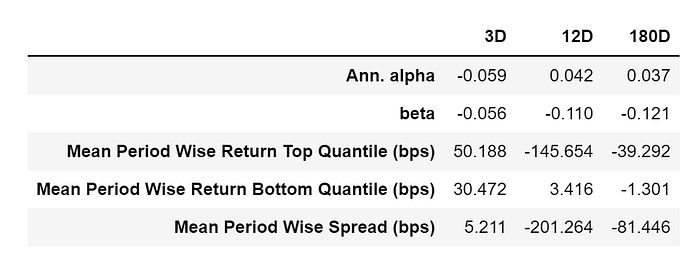
By applying the same approach to 30 Dow Jones stocks and the Nasdaq index, Dow Jones index had positive return to fscore relationship, while Nasdaq had negative return to fscore relationship. However, the number of stocks are substantially larger in the Nasdaq. As the focus of my paper is for the Hong Kong stock market. Below results are only for reference without further expansion
Dow Jones

Nasdaq
5.6 Industry level result in Hong Kong
Below filters were applied before computing the fscore return distribution in each GICS sub-industry.
- There must be equal or more than 2 companies in each industry
- Under each year of each industry, pb < 1. (pb < 999 yielded slightly better result but not statistically different)
- Under each year of each industry, company market cap must be less than 1 billion HKD
- One-fifth of both upper and lower end values are winsorized. (e.g. top and bottom two values in 10 samples are made equal to the second largest or lowest value.)
- Forward filling is used for calculating forward return
- HSI adjusted returns are calculated as the median for every two companies with fscores differences bigger than 6 or more in one industry.

By looking at the result summary, there are an average of 11.73 stocks in each industry. My strategy generated an average of 4.71 trades for each industry over the last decade. Due to the big tailed returns generated by low pb stocks, we should only look at 50% median statistics. So the median indicates on average, stock prices move in random walk with regard to fscores in the short run as all information is readily available for all analysts at all time. However, the strategy is able to shorten the realization of long term submartingale type of stock return, generating a median of 3.95% on top of the HSI index as well as being beta neutral. Implicitly, fundamentally strong firms with good fscore are expected to beat peers consistently in the long run. However at this point, it is indistinguishable if the return comes from other risks like financial distress or liquidity or etc.
(Sort by 3D return)

(Sort by 90D return)

The industry distribution of average returns based on fscore is not significantly shifted to the right. Moreover it is important to determine why some industries align negatively with the fscore. More specifically why would any return not follow fscore.
Section 6: Results
6.1 Company overview
To better understand the capability of my fscore strategy, I picked one specific long + short trade from the leisure products sub-industry (GICS code = 25201010) in the year of 2020, which generated undesired results.

Both companies are in the same market cap and pb tier range, who manufacture toys for the majority of the revenue.
Company price charts: (Green=Herald,Purple=Playmates)

6.2 Data verification
Before doing further analysis, I had to perform an item-by-item check on all the time, pricing, fundamental data, etc between few public sources and my code output. Evidence given in below excel screenshot.

*Yellow color represents positive factors, red color represents negative factors.
6.3 My factors
For the construction of each financial statement metric, readers can refer to section 5.3 of this paper or WRDS for more details. Fscore increases by one if each item below is true.
- F_ROA > 0. It is weighted by average yearly asset, and ‘below line items’ in the income statement are not considered.
df2.loc[‘incomebeforeextra’,:][i]/(0.5*(df2.loc[‘totalasset’,:][i]+df2.loc[‘totalasset’,:][i-1]))
- F_CFO > 0. Also weighted by average yearly asset
df2.loc[‘totalcashfromoperatingactivities’,:][i]/(0.5*(df2.loc[‘totalasset’,:][i]+df2.loc[‘totalasset’,:][i-1]))
- F_DELTAROA > 0. It is not weighted by average asset as it would need 3 year data points instead of 2.
df2.loc[‘incomebeforeextra’,:][i]/df2.loc[‘totalasset’,:][i]-df2.loc[‘incomebeforeextra’,:][i-1]/df2.loc[‘totalasset’,:][i-1]
- F_DELTAROA_BIG > 25% and F_DELTAROA > 0. In the case of extremely large ROA, I think it is significant enough to worth an additional point
df2.loc[‘incomebeforeextra’,:][i]/df2.loc[‘totalasset’,:][i]-df2.loc[‘incomebeforeextra’,:][i-1]/df2.loc[‘totalasset’,:][i-1])/abs(df2.loc[‘incomebeforeextra’,:][i-1]/df2.loc[‘totalasset’,:][i-1]
- F_ACCRUAL >0. Even for negative ROA and CFO.
F_CFO-F_ROA
- F_DELTALEVER <= 0. Zero long term debt is also considered good.
df2.loc[‘longtermdebt’,:][i]/df2.loc[‘totalasset’,:][i]-df2.loc[‘longtermdebt’,:][i-1]/df2.loc[‘totalasset’,:][i-1]
- F_LIQUID > 1.5. This threshold makes more sense than simply comparing ratio differences.
df2.loc[‘totalcurrentassets’,:][i]/df2.loc[‘totalcurrentliabilities’,:][i]
- EQ_OFFER <= 0. I considered various candidates for this metric, and eventually picked ‘salestock’.
df2.loc[‘salestock’,:][i]
- F_DELTAMARGIN > 0.05. It makes more sense to compare the increase ratio rather than difference for this item.
((df2.loc[‘totalrevenue’,:][i]-df2.loc[‘cogs’,:][i])/df2.loc[‘totalrevenue’,:][i]-(df2.loc[‘totalrevenue’,:][i-1]-df2.loc[‘cogs’,:][i-1])/df2.loc[‘totalrevenue’,:][i-1])/abs((df2.loc[‘totalrevenue’,:][i-1]-df2.loc[‘cogs’,:][i-1])/df2.loc[‘totalrevenue’,:][i-1])
- F_DELTATURN > 0.05. It makes more sense to compare the increase ratio rather than difference for this item.
(df2.loc[‘cogs’,:][i]/(0.5*(df2.loc[‘inventory’,:][i]+df2.loc[‘inventory’,:][i]-df2.loc[‘inventorychg’,:][i]))-df2.loc[‘cogs’,:][i-1]/(0.5*(df2.loc[‘inventory’,:][i-1]+df2.loc[‘inventory’,:][i-1]-df2.loc[‘inventorychg’,:][i-1])))/abs(df2.loc[‘cogs’,:][i-1]/(0.5*(df2.loc[‘inventory’,:][i-1]+df2.loc[‘inventory’,:][i-1]-df2.loc[‘inventorychg’,:][i-1])))
6.4 Other unused potential factor candidates
- stock repurchase
REPURCHASE = df2.loc[‘repurchase’,:][i]-df2.loc[‘repurchase’,:][i-1]
- prefer less popularity and analyst coverage
POPULARITY = (df2.loc[‘volume’,:][i]-df2.loc[‘volume’,:][i-1])/df2.loc[‘volume’,:][i-1]
- For good economy, prefer good momentum for the low pb stocks as good performance tend to keep rising
MOMENTUM1 = (df2.loc[‘close’,:][i]-df2.loc[‘close’,:][i-1])/df2.loc[‘close’,:][i-1]
- short stocks with extreme increase in pb
MOMENTUM2 = (df2.loc[‘close’,:][i]-df2.loc[‘close’,:][i-1])/df2.loc[‘close’,:][i-1]
6.5 Other calculated metrics
- df2.loc[‘pb’][i] = df2.loc[‘close’,:][i]*df2.loc[‘sharesos’,:][i]/(df2.loc[‘commonequity’,:][i]*(1000000))
- df2.loc[‘pe’][i] = df2.loc[‘close’,:][i]*df2.loc[‘sharesos’,:][i]/(df2.loc[‘incomebeforeextra’,:][i]*(1000000))
- df2.loc[‘mcap’][i] = df2.loc[‘close’,:][i]*df2.loc[‘sharesos’,:][i]/(1000000)
- df2.loc[‘ROA’][i] = df2.loc[‘incomebeforeextra’,:][i]/(0.5*(df2.loc[‘totalasset’,:][i]+df2.loc[‘totalasset’,:][i-1]))
- df2.loc[‘ACCRUAL’][i] = F_CFO-F_ROA
- df2.loc[‘LEVER’][i] = df2.loc[‘longtermdebt’,:][i]/(0.5*(df2.loc[‘totalasset’,:][i]+df2.loc[‘totalasset’,:][i-1]))
- df2.loc[‘LIQUID’][i] = df2.loc[‘totalcurrentassets’,:][i]/df2.loc[‘totalcurrentliabilities’,:][i]
- df2.loc[‘MARGIN’][i] = (df2.loc[‘totalrevenue’,:][i]-df2.loc[‘cogs’,:][i])/df2.loc[‘totalrevenue’,:][i]
- df2.loc[‘TURN’][i] = 360/(df2.loc[‘cogs’,:][i]/(0.5*(df2.loc[‘inventory’,:][i]+df2.loc[‘inventory’,:][i]-df2.loc[‘inventorychg’,:][i])))
- df2.loc[‘EQ_OFFER’][i] = df2.loc[‘salestock’,:][i]
- df2.loc[‘D/A’][i] = df2.loc[‘totalliabilities’,:][i]/df2.loc[‘totalasset’,:][i]
*For the details of company book value calculation see [3] in the references section.
6.6 Cross-sectional result
In the 2020 leisure industry cross-sectional result, it is inconclusive to say high fscore companies perform better than low fscore companies in the 90D future, because companies exist through time. Company A with score 8 is better, compared to company B with score 2, but company A with score 8 is worse compared to company A with score 9 in the previous year.
6.7 Time series result
The spread between 0114 and 0869 started to widen after 2019, measured by linear regression rolling residual.

Time series comparison between 0114 (BMG4410A1062) and 0869 (BMG7147S1008) is depicted in the following screenshot. This is the utmost important result in this entire study. According to the highlighted rows, returns are realized previous to companies reporting high fscore financial statements, rather than afterwards. I think there are two main drivers for the unprofitable holistic result in section 5.4 of this paper according to longing high fscore and shorting low fscore companies:
- Good financial statements are the result rather than the cause of good company performance. In the digital age, good news is always rewarded quickly as markets become more and more efficient.
- Especially for the low pb, small, low liquidity, and low analyst coverage stocks, there would be more professional, and less speculative traders. This leads to more likelihood of insider trading without immediately publication of important news.

Section 7: Company fundamental analysis
7.1 Overview:
Herald (http://0114.HK) and Playmates (http://0869.HK) are traditional toys manufacturers in Hong Kong. Apart from toy manufacturing which offers nearly 70% total revenue, Herald has other businesses like Computer Products, Housewares, Timepieces and other investments. The Computer Products division and Timepieces division provide 11% and 13% of revenue in 2019–2020 respectively. Playmate’s main business is toy manufacturing, which needs to acquire licenses from major studios and animated series, and its famous iconic toys are Teenage Mutant Ninja Turtles and Disney’s Frozen2 Figures.

7.2 Profitability analysis
Here interim financial statement data is also considered as previously paper only considered annual data.
(http://0114.hk Herald Holdings Limited)
Sep-20Mar-20Sep-19Mar-19Sep-18Mar-18InterimAnnualInterimAnnualInterimAnnualROE2.98%1.27%-0.89%-3.57%-5.90%-3.47%Net profit margin3.55%0.73%-1.30%-2.94%-8.26%-2.35%CoGS to revenue ratio77.96%79.07%79.67%85.27%86.89%80.01%SG&A expense to revenue ratio18.47%21.19%19.53%23.78%23.53%23.14%
(http://0869.hk Playmates Toys Limited)
Jun-20Dec-19Jun-19Dec-18Jun-18InterimAnnualInterimAnnualInterimROE-5.49%-3.72%-1.97%0.05%-2.98%Net profit margin-62.64%-10.39%-12.66%0.12%-22.34%CoGS to revenue ratio53.94%48.64%49.09%47.09%52.82%SG&A expense to revenue ratio72.08%38.87%44.88%31.49%50.15%
In equally bad times, Herald has been good at turning losses into profit by improving both cost and expenses, especially in selling general and administrative expenses. In contrast, Playmates’ cost management has been getting worse, and couldn’t generate any positive returns since 2018 FY.
Section 8: Next Steps and challenges
This paper needs more in-depth analysis on the relationship between companies fundamentals and market reaction by reading full financial statements and footnotes, especially after 2019 when spread between 0114 and 0869 widened.
In my analysis I realized it was challenging to match fscore performance with realized return. pb ratios are relatively more stable than pe ratios across time. However it takes more research to fully understand the best use of pe ratio corresponding to the fscore strategy. A high pe ratio can mean very little earnings; a negative pe ratio can both mean upward potential or degrading performance; when earnings shrink, both price and book value shrink as well.
If faced with industries of more competitors, the strategy could also be used to arbitrage pb ratio on stocks with the same fscore. By arbitraging this way, it removes the time series effect for each company as the previous price was already taken into account. Doing this cross-sectionally can further bet if the market can fairly price the same industry stocks at one point of time.
Strategy works better on companies with more similar business models rather than conglomerates.
There is little mention of statistical tests in my paper because I believe conviction in this strategy comes from stories behind each financial statement. Average return and standard deviation among industries have no value outside of statistics. It is also hard to explain the collinearity effect among different years of economy. However I have used some techniques similar as bootstrapping or fama-macbeth to average cross sectional data on top of time series.
Section 9: Conclusion
Abnormal return can only be realized before good fundamental performance is revealed to the public, but not afterwards. Details see main result section in 6.7.
Reference:
[1] Piotroski, J. (2000). Value Investing: The Use of Historical Financial Statement Information to Separate Winners from Losers. Journal of Accounting Research, 38, 1–41. doi:10.2307/2672906
[2] Eremenko, Egor, Quantitative Fundamentals. Application of Piotroski F-Score on Non-U.S. Markets. (April 9, 2017). Available at SSRN: https://ssrn.com/abstract=3262154 or http://dx.doi.org/10.2139/ssrn.3262154
[3] Ray Ball, Joseph Gerakos, Juhani T. Linnainmaa, Valeri Nikolaev,
Earnings, retained earnings, and book-to-market in the cross section of expected returns, Journal of Financial Economics, Volume 135, Issue 1, 2020, Pages 231–254, ISSN 0304–405X, https://doi.org/10.1016/j.jfineco.2019.05.013. (http://www.sciencedirect.com/science/article/pii/S0304405X19301382) Abstract: Book value of equity consists of two economically different components: retained earnings and contributed capital. We predict that book-to-market strategies work because the retained earnings component of the book value of equity includes the accumulation and, hence, the averaging of past earnings. Retained earnings-to-market predicts the cross section of average returns in U.S. and international data and subsumes book-to-market. Contributed capital-to-market has no predictive power. We show that retained earnings-to-market, and, by extension, book-to-market, predicts returns because it is a good proxy for underlying earnings yield (Ball, 1978; Berk, 1995) and not because book value represents intrinsic value.